It is easy to make a depreciation worksheet in Excel without using complex and conditional formulas. You only need to familiarize yourself with the SLN
Straight-line method
, DDB
Double-declining balance method
, and SYD
Sum-of-the-years digits method
formulas to compute depreciation.
Featured Partner
Fit Small Business is able to offer our services for free because some vendors may pay us for web traffic or other sales opportunities. Our mission is to help technology buyers make better purchasing decisions, so we provide you with information for all vendors — even those that don’t pay us.
1
Acumatica Cloud ERP
Employees per Company Size
Micro (0-49), Small (50-249), Medium (250-999), Large (1,000-4,999), Enterprise (5,000+)
Any Company Size
Any Company Size
Features
Accounts Receivable/Payable, API, Departmental Accounting, and more
I’ll show you how I built a depreciation worksheet from scratch, from setting up column headers to entering formulas and using each depreciation method. I have also included a free downloadable template you can start using right away, in case you want to skip the whole process I show below.
![How To Make a Depreciation Worksheet in Excel [+Template]](https://fitsmallbusiness.com/wp-content/uploads/2024/03/Screenshot_of_Depreciation_Computation.jpg "How To Make a Depreciation Worksheet in Excel [+Template]")
Thank you for downloading!
The images shown in my step-by-step tutorial are for demonstration purposes only and will not match my downloadable template.
Hopefully, by walking you through how to make a depreciation worksheet in Excel, you’ll learn how to customize my downloadable template to suit your needs.
Step 1: Assemble the column headers in row 1.
Here’s how I set up the depreciation worksheet in Excel. First, I created a new Excel spreadsheet and entered the following column headers in row 1:
- Asset’s Name
- Useful Life
- Historical Cost
- Salvage Value
- Current Period
- Depreciation Expense
- Accumulated depreciation, beginning
- Accumulated depreciation, ending

What your spreadsheet should look like
Row 1 serves as the column headers, so I ensured that they’re labeled clearly. I also adjusted the column widths to leave enough space for the data.
For values in Columns B, C, F, G, and H, I formatted the cells as Currency so that they display the dollar sign. To do this, follow this process:
- Right-click on the cell or column.
- Select Format Cells.
- Go to the Currency category.
- Choose the desired format (e.g., 2 decimal places, symbol: $).
This formatting step keeps the worksheet clean and easy to read.
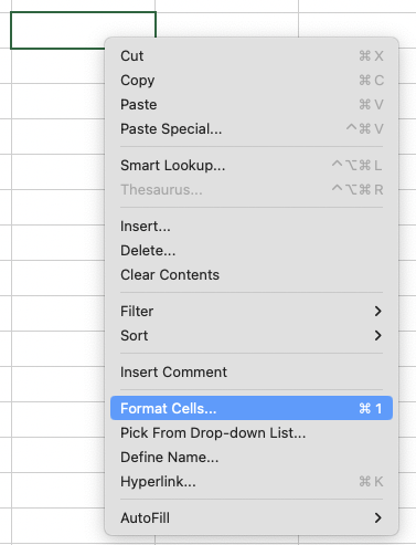
Shortcut To Format Cells
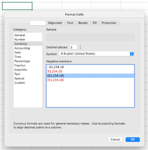
Format cell values as currency
The blue cells in my downloadable template are for data entry, and this is where I input the asset details and other values. Meanwhile, the gray cells already contain built-in formulas, so I let the gray cells do the work. This keeps everything running smoothly and prevents errors in the calculations.

Worksheet in our downloadable template
You can always download the template I made if you think it’s a hassle to create one from scratch. But if you’d like to brush up on your Excel skills, read on!
Where to get the data
The easiest way I get fixed asset data is by generating a report from my accounting software. I look for a report that shows all activity in the fixed asset balance sheet accounts.
By reviewing this report, I can usually find the cost of the asset and the purchase date. For the useful life and salvage value, I check if there’s any documentation that outlines standard values for different fixed asset types. This might come from internal policies or previous asset schedules.
Step 2: Enter the depreciation expense formulas.
The depreciation formula may differ depending on what method you use. Regardless of the method, enter the formula in Column F of the worksheet.
Here are the syntaxes of the different depreciation formulas you can use:
Syntax: =SLN(cost, salvage, life)
- Cost (required) is the historical cost of the asset.
- Salvage (required) is the salvage value of the asset. If none, place zero.
- Life (required) is the useful life of the asset.

How you insert the arguments for SLN
The cost of the asset, salvage value, and useful life are in cells B2, C2, and D2, respectively. Hit Enter after completing all arguments.
There are two common variations of the declining balance method. You can either use double-declining or 150% declining by using just one syntax.
Syntax: =DDB(cost, salvage, life, period, [factor])
- Cost (required) is the historical cost of the asset.
- Salvage (required) is the salvage value of the asset. If none, place zero instead.
- Life (required) is the useful life of the asset.
- Period (required) is the point in time for which you want to compute depreciation. It must be the same units as life, such as if life is in years, then the period can be 1 for the first year, 2 for the second year, and so on.
- Factor (optional) is the rate at which depreciation declines.
- If omitted, Excel uses 2 or 200% declining rate.
- If you want to use 150% declining, add 1.5 to the factor argument.

How you add the arguments for 200% declining balance

How you add the arguments for 150% declining balance
Syntax: =SYD(cost, salvage, life, per)
- Cost (required) is the historical cost of the asset.
- Salvage (required) is the salvage value of the asset. If none, place zero instead.
- Life (required) is the useful life of the asset.
- Per (required) is the point in time for which you want to compute depreciation, such as 1 for first year or 10 for 10th year.

How you insert the arguments for SYD
The current period is 2, which means we want to know the sum-of-the-years depreciation for the second year.
In the template I created, the worksheet automatically selects the correct depreciation formula based on a set of conditions. So, there’s no need for you to enter the formula in each row manually.
Still, the template uses the same depreciation methods I explained earlier: SLN, DDB, and SYD. I recommend getting familiar with how each formula works, especially if you plan to make changes or customize the template. Understanding the logic behind the template gives you more flexibility and control.
Step 3: Enter the accumulated depreciation formulas.
To get started, I pulled up last year’s depreciation worksheet, so go ahead and do the same. I copied the ending Accumulated Depreciation for each fixed asset and pasted it into this year’s beginning Accumulated Depreciation column.
If you don’t have a previous worksheet, generate a report from your accounting software that shows the beginning Accumulated Depreciation for each asset. If that’s unavailable, you’ll have to compute the beginning balance manually.

What accumulated depreciation for one sample asset looks like
In Cell H2, I enter the formula =F2+G2 to calculate the ending Accumulated Depreciation. This adds the Depreciation Expense (F2) and the beginning Accumulated Depreciation (G2).
To apply this formula to the rest of the rows, I used Excel’s autofill feature. I clicked on Cell H2, then hovered my cursor over the bottom right corner until I saw a small square. Once it appeared, I clicked and dragged it down to fill the formula in the rows below.
Frequently asked questions (FAQs)
A depreciation worksheet is a document that shows the depreciation expense and accumulated depreciation of an asset. It lets you track depreciation for the current year and serves as an internal reference document for depreciation journal entries.
The formulas you need to familiarize yourself with are SLN, DDB, and SYD. The syntax of each formula is as follows:
- SLN: =SLN(cost, salvage, life)
- DDB: =DDB(cost, salvage, life, period, [factor])
- SYD: =SYD(cost, salvage, life, per)
The formula depends on the depreciation method used.
- Straight-line depreciation: (Cost − SalvageValue) ÷ Useful Life
- Double declining balance: BookValue × ( 2 ÷ Useful Life)
- Sum-of-years’ digits: (Remaining Life ÷ Sum of the Years) × (Cost − Salvage Value)